Manual
Data Types
There are five main data formats used within CNSistent.
The SCNA data are stored in cns_df.
Sample metadata are stored in samples_df.
BAM files are converted into segments and mapped per chromosome.
Internally, breakpoints are used for collecting per chromosomes breakpoints.
For reference, the Assembly class is used to provide information about the genome.
cns_df
A pandas DataFrame with the following columns:
sample_id, chrom, start, end, CN, .... TheCNcolumns are the copy number values for each segment. Thechromcolumn is expected to be in the formatchr1,chr2, …,chrX,chrY,chrM. Thestartandendcolumns are 0-based coordinates.
sample_id  chrom     start       end  CN1  CN2
0        s1  chr19         0  13000000    1    1
1        s1  chr19  13000000  59128983    3    1
2        s2  chr19         0  26500000    2    0
3        s2  chr19  26500000  59128983    0    0
samples_df
A pandas DataFrame with the following columns:
sample_id, sex. Thesexcolumn is expected to bexyorxx.sex sample_id s1 xx s2 xy
segments
A dictionary of lists with keys being chromosomes and each segment being 0-indexed triples of start and end coordinates and a string id.
{'chr19': [(0, 13000000, 'chr19_0'), (13000000, 26500000, 'chr19_1'), (26500000, 59128983, 'chr19_2')]}
breakpoints
A dictionary of lists with keys being chromosomes and each breakpoint being a 0-indexed position in the chromosome.
{'chr19': [0, 13000000, 26500000, 59128983]}
Assembly
Assembly is a class that provides information about the species.
CNSistent currently supports hg19 and hg38 assemblies. If you want to use it with a different assembly, you need to create a new object.
Note that sex chromosomes are always expected to be named chrX and chrY.
Assembly(name, chr_lens, chr_x, chr_y, gaps, cytobands)
chr_lensis a dictionary with chromosome names as keys and lengths as values. Thechr_xandchr_yarechr_x,chr_yare the string ids for sex chromosomes. “chrX” and “chrY” are used by default.gaps,cytobandsare segment dictionaries for gaps and cytobands, respectively.
These can be null unless you use regions_select("bands") or regions_select("gaps").
Pipelines
Pipelines are used internally to map the command line commands and arguments to functions, and thus correspond to Tool usage (CLI). Each command has a corresponding pipeline. In addition, two combined pipelines are provided as shorthands.
main_impute: Will align the missing regions and infer the missing values.main_seg_agg: Will create and apply segmentation.
See the tutorial for examples of how to use the pipelines.
Segmentation
CNSistent operates over segments. Segments are dictionaries of tuples {chr: [(start, end, name), ...], ...}, where the start is inclusive, and the end is exclusive.
Note that you can pass longer tuples, but the result will discard the 4th and further elements.
The following functions can be used to manipulate segments:
split_segments: Will split into equidistant chunks based on specified size (useful for binning).merge_segments: Will merge overlapping segments, merging is possible ifend==startfor two consecutive segments on the same chromosome. Note that if the segments are not sorted, you need to setsort=Trueto sort them first.segment_union: Will merge segments from two lists of segments.get_consecutive_segs: Having a list of segments, creates lists of consecutive segments.segment_difference: Will remove regions from a list of segments found in another list of segments.regions_select: A versatile function for creation of segments, seeregions_select.filter_min_size: Will remove segments strictly smaller than the specified size.
Imputation
Functions for adding missing segments and values in the CNS data. The process is to first add missing regions with NaN values and then impute the missing values.
There are separate functions to fill the telomeres, fill the gaps, and add missing chromosomes.
If guessing values in imputation is not desired, the fill_nans_with_zeros function can be used to simply fill with 0 instead.
Clustering
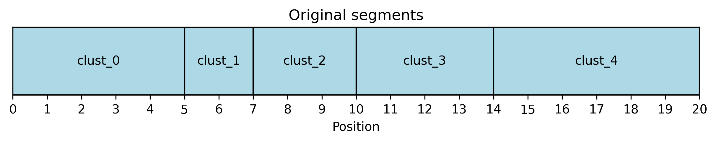
Clustering merges neigbouring breakpoints. The breakpoints are then merged using a greedy algorithm on a predefined region (usually a whole chromosome). Starting from the leftmost breakpoint, all breakpoints within the merge distance m are accumulated and a new breakpoint is created as their average. This is then repeated from the leftmost not yet merged breakpoint, until the end of the region is reached.
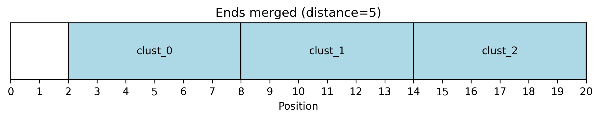
Clustering can either preserve endpoints (and only merge internal breakpoints), or also merge the endpoints. Example on list [0, 5, 7, 10, 16, 20] with merge distance 5:
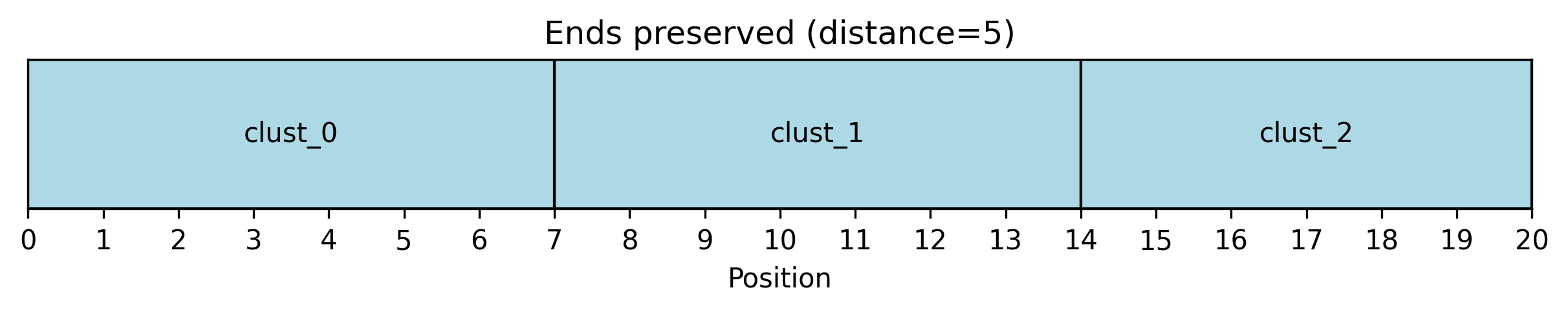
> When using aggregation with clustering, the endpoints are always preserved.
Aggregation
Aggregation will produce segments of a certain size, aggregating the copy number values of the segment chunks into a single segment.
There are the following aggregate functions: mean, min, max, and none. The none function will just split existing bins, without additional aggregation. This is useful if you want to introduce additional breakpoints into the data.
Aggregation can be done either using explicit segments, explicit breakpoints, or a breakpoint type (e.g. arms, 1000000).
Analyze
The analyze module calculates statistics for the CNS data.
coverage: Calculates the proportion of genome with assigned (not NaN) CN values.ploidy: Calculates the proportion of genome with aneuploid CN values (different from 2 or 1 for male sex chromosomes).breakage: Calculates the signatures related statistics ` currently it only calculates breakpoints per sample/chromosome.
Plotting
Display functions are in three categories:
fig: A Whole figure with labels.plot: Takes an axis and plots on it.labels: Takes an axis and adds background / ticks.
For the figures, the first parameter is always the CNS_df, or a list thereof in the case of joint plots.
There is one feature (line, dots…) per sample_id and one plot per cn_column.
Following optional parameters: * cn_columns: a string describing the column to plot or a list thereof. If none is specified, all columns matching the CN column pattern are used. * chrom: a string describing the chromosome to plot. If none is specified, all chromosomes are used. * size: Size of the feature of the plot - line/boundary width or dot size.
Examples can be found in the plotting notebook.
Utils
Utils contain the specification for the hg19, hg38 assemblies, including the gaps and cytobands. In addition, functions for files and data are provided:
Files
load_cns/save_cns: Load/Save CNS data from a TSV file, with optional header and sample_id. By default, this moves from 1-based to 0-based coordinates.load_regions/save_regions: Load/Save regions from a TSV file, reading only thechrom, start, endcolumns. By default, this moves from 1-based to 0-based coordinates.load_samples/save_samples: Load samples from a TSV file. The first column is used as “sample_id” index and should match the CNS sample names.get_cn_columns: Get the CN columns from a CNS DataFrame (start or end withCNorcn).
Selection
Functions to select samples set from CNS df (head, tail, random), to filter chromosomes (autosomes, sex chromosomes…) and samples/CNS by type.
Conversions
Converts between CNS df, breakpoints, and segments.
Data Utils
Functions to load the datasets (PCAWG, TCGA, TRACERx) and gene sets (Ensembl, COSMIC).
Default filtering to remove samples from the datasets (low coverage, diploid, blacklisted, …)
Loading binned data / processed samples.