Examples: Plotting

Below are examples of data aggregation and plotting functions that can be used to visualize the data.

[1]:

import cns
import cns.data_utils as cdu
import matplotlib.pyplot as plt

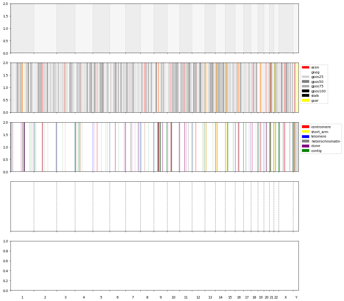
Labeling functions

These functions create background/s labels independent of the data.

[2]:

fig, axs = plt.subplots(5,1, figsize=(15, 15), sharex=True, dpi=50)
cns.plot_chr_bg(axs[0])

cns.plot_cytobands(axs[1], alpha=.25)
cns.add_cytoband_legend(axs[1])

cns.plot_gaps(axs[2], alpha=.25)
cns.add_gap_legend(axs[2])

cns.plot_x_ticks(axs[3])
cns.plot_x_lines(axs[3])
cns.no_y_ticks(axs[3])

Prepare Data

Loads and aggregates the data.

[3]:

pcawg_cns_df = cns.add_total_cn(cdu.load_cns_file("PCAWG_cns_imp.tsv"))
pcawg_cns_df.head()

[3]:

	sample_id	chrom	start	end	major_cn	minor_cn	total_cn
0	SP101724	chr1	0	27256755	2.0	2.0	4.0
1	SP101724	chr1	27256755	28028200	3.0	2.0	5.0
2	SP101724	chr1	28028200	32976095	2.0	2.0	4.0
3	SP101724	chr1	32976095	33354394	5.0	2.0	7.0
4	SP101724	chr1	33354394	33554783	3.0	2.0	5.0

[4]:

genes_segs = cdu.load_segs_out("segs_COSMIC.bed")

pcawg_1_bin_df = cns.aggregate_by_break_type(cns.cns_head(pcawg_cns_df, 1), 100_000)
pcawg_1_groups_df = cns.group_samples(pcawg_1_bin_df, group_name="100 kb")

pcawg_10_bin_df = cns.aggregate_by_break_type(cns.cns_head(pcawg_cns_df, 10), 1_000_000)
pcawg_10_groups_df = cns.group_samples(pcawg_10_bin_df, group_name="1 mb")

pcawg_50_bin_df = cns.aggregate_by_break_type(cns.cns_head(pcawg_cns_df, 50), 10_000_000)
pcawg_50_groups_df = cns.group_samples(pcawg_50_bin_df, group_name="10 mb")

pcawg_arms_bin_df = cns.aggregate_by_break_type(cns.cns_head(pcawg_cns_df, 10), "arms")
pcawg_arms_groups_df = cns.group_samples(pcawg_arms_bin_df, group_name="arms")

gene_bin_df = cns.aggregate_by_segments(cns.cns_head(pcawg_cns_df, 10), genes_segs)
gene_groups_df = cns.group_samples(gene_bin_df, group_name="COSMIC")

Aggregated into 30363 CNS.
Aggregated into 30399 CNS.
Aggregated into 15256 CNS.
Aggregated into 462 CNS.
Aggregated into 7220 CNS.

Plots

[5]:

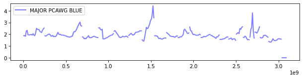
fig, ax = plt.subplots(1, 1, figsize=(10, 2), dpi=75)
cns.plot_lines(ax, pcawg_50_groups_df, "major_cn", "blue", "MAJOR PCAWG BLUE", .5, 2)
ax.legend()

[5]:

<matplotlib.legend.Legend at 0x1c470c49d50>

[6]:

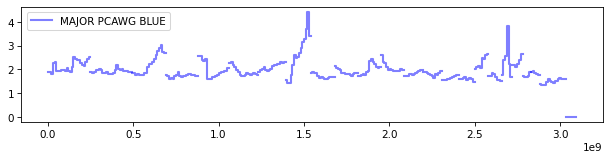
fig, ax = plt.subplots(1, 1, figsize=(10, 2), dpi=75)
cns.plot_steps(ax, pcawg_50_groups_df, "major_cn", "blue", "MAJOR PCAWG BLUE", .5, 2)
ax.legend()

[6]:

<matplotlib.legend.Legend at 0x1c46c92d3d0>

[7]:

fig, ax = plt.subplots(1, 1, figsize=(10, 2), dpi=75)
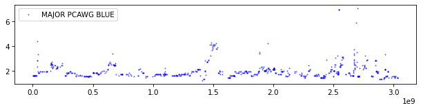
cns.plot_dots(ax, gene_groups_df, "major_cn", "blue", "MAJOR PCAWG BLUE", .5, 1)
ax.legend()

[7]:

<matplotlib.legend.Legend at 0x1c470558b50>

[8]:

fig, ax = plt.subplots(1, 1, figsize=(10, 2), dpi=75)
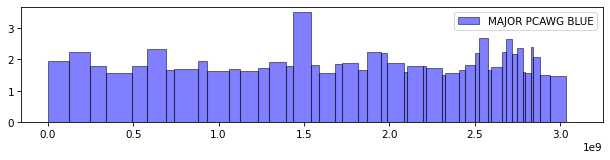
cns.plot_bars(ax, pcawg_arms_groups_df, "major_cn", "blue", "MAJOR PCAWG BLUE", .5)
ax.legend()

[8]:

<matplotlib.legend.Legend at 0x1c47f812690>

[9]:

fig, ax = plt.subplots(1, 1, figsize=(10, 2), dpi=75)
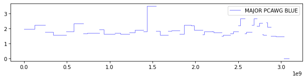
cns.plot_steps(ax, pcawg_arms_groups_df, "major_cn", "blue", "MAJOR PCAWG BLUE", .5)
ax.legend()

[9]:

<matplotlib.legend.Legend at 0x1c470558e50>

[10]:

fig, ax = plt.subplots(figsize=(10, 2), dpi=75)
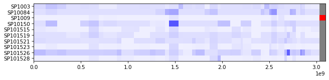
cns.plot_heatmap(ax, pcawg_arms_bin_df, "major_cn", max_cn = 16)

[10]:

<Axes: >

Figures

[11]:

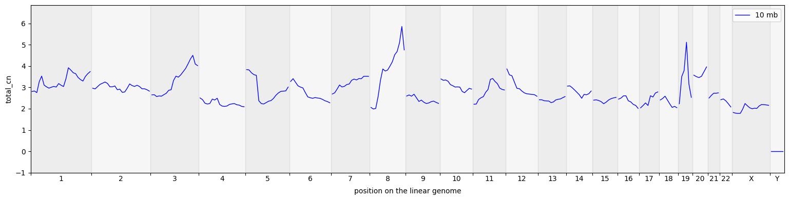
cns.fig_lines(pcawg_50_groups_df, cn_columns="total_cn", colors="blue");

[12]:

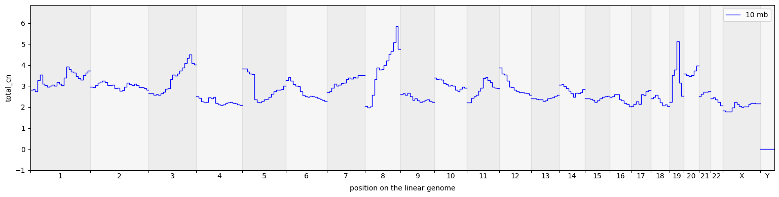
cns.fig_steps(pcawg_50_groups_df, cn_columns="total_cn");

[13]:

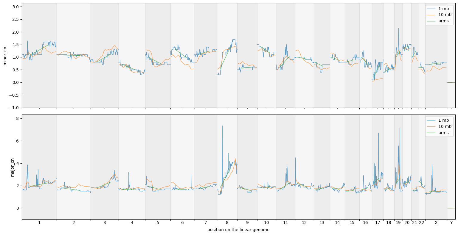
groups_df = cns.stack_groups([pcawg_10_groups_df, pcawg_50_groups_df, pcawg_arms_groups_df])
cns.fig_lines(groups_df, cn_columns=["minor_cn", "major_cn"]);

[14]:

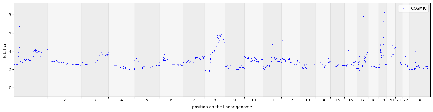
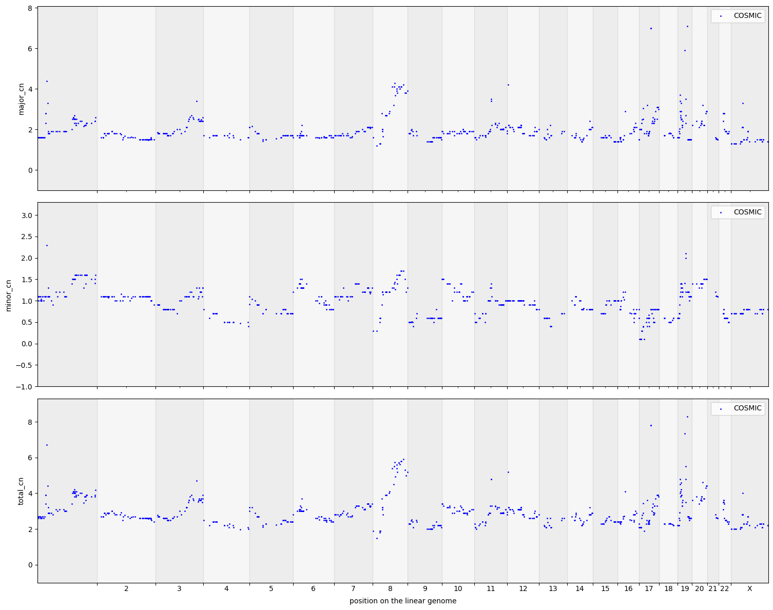
cns.fig_dots(gene_groups_df, cn_columns="total_cn");

[15]:

cns.fig_dots(gene_groups_df)

[15]:

(<Figure size 1516.62x1200 with 3 Axes>,
 array([<Axes: ylabel='major_cn'>, <Axes: ylabel='minor_cn'>,
        <Axes: xlabel='position on the linear genome', ylabel='total_cn'>],
       dtype=object))

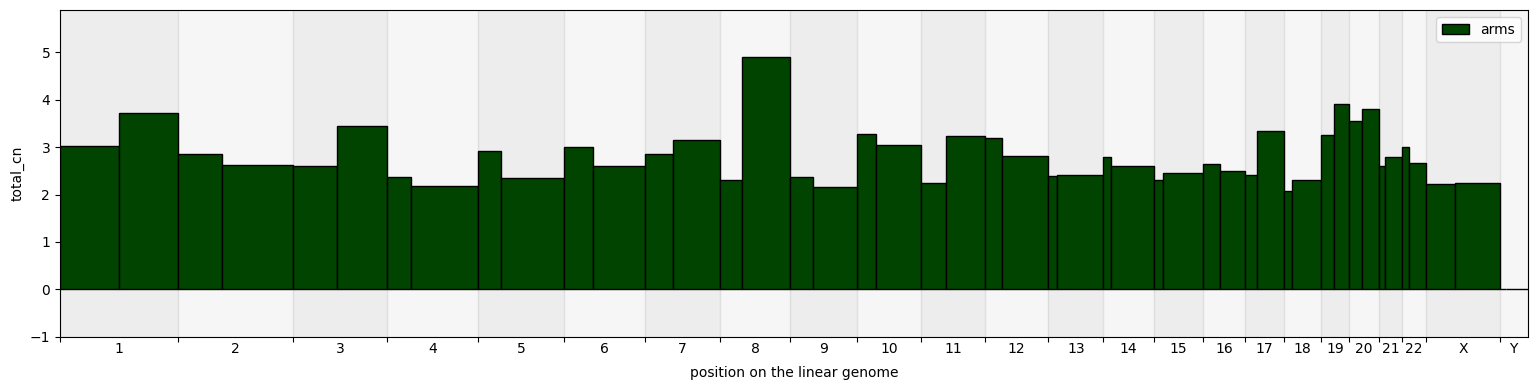
[16]:

cns.fig_bars(pcawg_arms_groups_df, cn_columns="total_cn", colors="#004400");

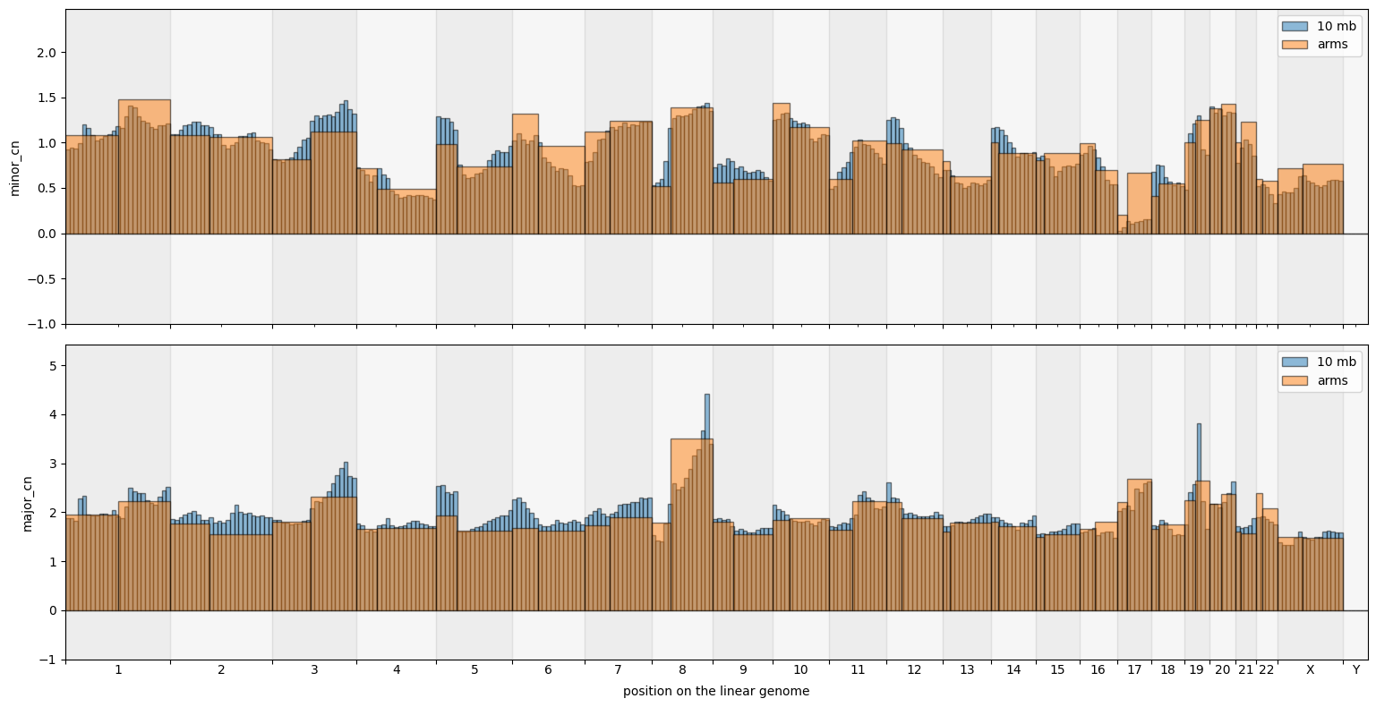
[17]:

big_groups = cns.stack_groups([pcawg_50_groups_df, pcawg_arms_groups_df])
cns.fig_bars(big_groups, cn_columns=["minor_cn", "major_cn"])

[17]:

(<Figure size 1547.84x800 with 2 Axes>,
 array([<Axes: ylabel='minor_cn'>,
        <Axes: xlabel='position on the linear genome', ylabel='major_cn'>],
       dtype=object))

Filter for single chromosome

[18]:

step = int(1e6)
segs = cns.main_segment(remove_segs=cns.make_segments("gaps"), split_size=step, filter_size=step//2)
filtered_cns = cns.main_aggregate(cns.cns_head(pcawg_cns_df, 10), segs=segs, cn_columns="major_cn")

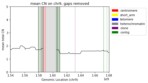
[19]:

grouped_bins = cns.group_samples(filtered_cns).query("chrom == 'chr9'")
fig, ax = plt.subplots(1, 1, figsize=(6, 4), dpi=75)
cns.plot_gaps(ax, alpha=.25, y_max=5)
cns.add_gap_legend(ax)
cns.plot_lines(ax, grouped_bins, "major_cn", color="black")
ax.set_xlim(*cns.x_limits(grouped_bins))
# no_y_ticks(ax)
ax.set_ylabel("mean total CN")
ax.set_xlabel("Genomic Location (chr9)")
ax.set_title("mean CN on chr9, gaps removed")
cdu.save_doc_fig("fig_gaps_removed_chr9")

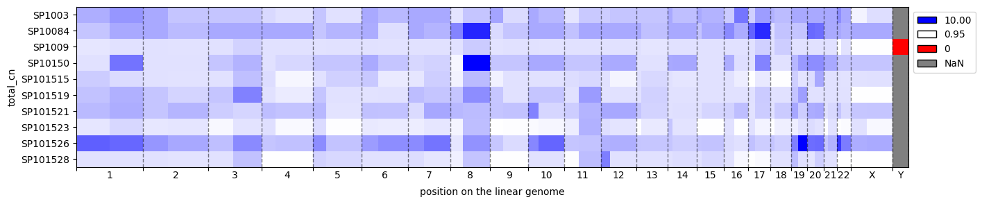
CN Heatmaps

[20]:

cns.fig_heatmap(pcawg_arms_bin_df, cn_columns="total_cn")

[20]:

(<Figure size 1547.84x300 with 1 Axes>,
 <Axes: xlabel='position on the linear genome', ylabel='total_cn'>)

[21]:

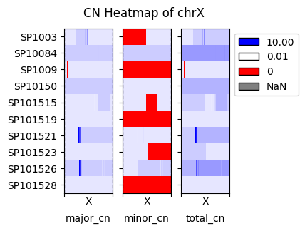
fig, axs = cns.fig_heatmap(pcawg_10_bin_df.query("chrom == 'chrX'"), max_cn=10, vertical=False)
fig.suptitle("CN Heatmap of chrX")

[21]:

Text(0.5, 0.98, 'CN Heatmap of chrX')